MO-210 Exam Preparation Material | Microsoft Excel (Microsoft 365 Apps)

Prepare for the MO-210 with reliable study materials, practice questions, and key exam insights.

Prepare for the MO-210 Microsoft Excel (Microsoft 365 Apps) exam with CertQueen's independently developed study resources. Review important concepts, practice scenario-based questions, and use clear explanations to identify areas that require further study.

Question#1

SIMULATION
Instructions
Exam Environment
Exam Interface and Controls
The exam panel provides access to the project task(s). Each project has an associated file in which you will perform the project tasks.

Overview:
Motorhome Rentals
Your company rents motorhomes. The motorhomes rent year-around at different prices. You are preparing pricing worksheets to be shared with others.
Task5:
On the Rentals worksheet, configure the heading row in the table so that entries wider than the column wrap to multiple lines.

A. To ensure that the text in your heading row (the table headers) is fully visible without changing the column width, you will use the Wrap Text feature.

Step-by-Step Solution
✑ Select the Header Row: In your "Rentals" worksheet, click and drag to select the cell rangeA2: F2(the orange heading row containing "Capacity," "Fleet Name," etc.).
✑ Navigate to the Home Tab: Ensure you are on the Home tab of the Ribbon .
✑ Apply Wrap Text:
✑ Verify the Result: The text in your headers will now automatically wrap to multiple lines if it exceeds the current width of the column.

Question#2

SIMULATION
Instructions
Exam Environment
Exam Interface and Controls
The exam panel provides access to the project task(s). Each project has an associated file in which you will perform the project tasks.

Overview:
Guitar Stores
You and a partner own several Guitar Stores. You are analyzing your revenue from the past two quarters.

Task 1:
On the Qtr 2 worksheet, in cell F10, insert a column sparkline showing the sales trend from Apr through Jun. Apply Gold, Sparkline Style Accent 2, Darker 25% to the sparkline. Copy the sparkline to the remaining cells in the column, F11: F14.

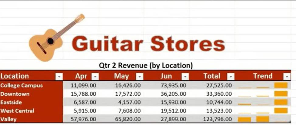
A. here is the step-by-step solution for Task 1:

Step 1: Navigate to the Correct Worksheet
Click on the Qtr 2worksheet tab at the bottom of the Excel window to ensure you are working on the correct data set.

Step 2: Insert the Column Sparkline
✑ Click on cellF10(this is where the first sparkline will reside).
✑ Go to the Insert tab on the Ribbon.
✑ In the Sparklines group, click on Column.
✑ A dialog box will appear. For Data Range, select the cells representing Apr through Jun for the first row (likelyB10: D10).
✑ Ensure the Location Range is set to$F$10.
✑ Click OK.

Step 3: Apply the Specific Sparkline Style
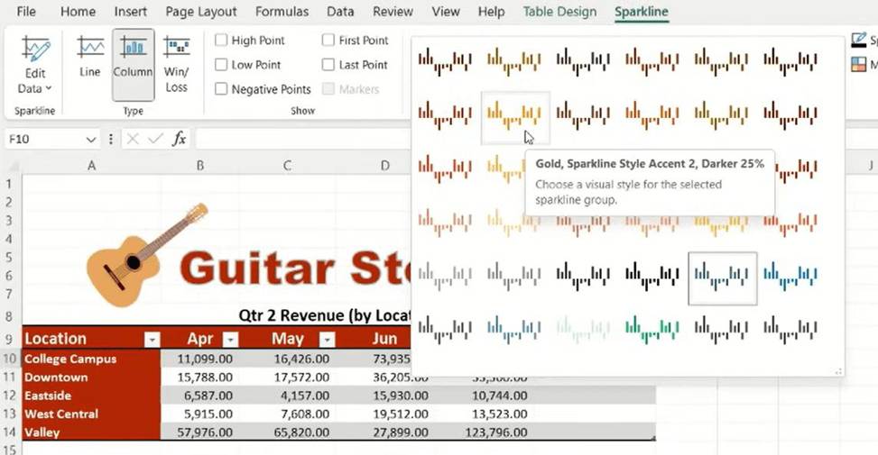
With cellF10still selected, a new Sparkline tab will appear at the top of your Ribbon.
✑ Click on the Sparkline tab.
✑ Click the More arrow (the small downward arrow at the bottom right) of the Styles gallery to see all options.
✑ Hover over the styles to find the specific name: Gold, Sparkline Style Accent 2, Darker 25%.
✑ Click to apply it.

Step 4: Copy the Sparkline to Remaining Cells
✑ Select cellF10.
✑ Hover your mouse over the Fill Handle (the small green square in the bottom-right corner of the cell).
✑ Click and drag the handle down to cellF14.
✑ Excel will automatically generate sparklines for the other locations (Downtown, Eastside, etc.) using the same style and corresponding data rows.

Question#3

SIMULATION
Instructions
Exam Environment
Exam Interface and Controls
The exam panel provides access to the project task(s). Each project has an associated file in which you will perform the project tasks.

Overview:
Motorhome Rentals
Your company rents motorhomes. The motorhomes rent year-around at different prices. You are preparing pricing worksheets to be shared with others.

Task 2:
Add the value New Rates to the Title property of the document.

A. To add a value to the Title property of an Excel document, you need to access the Backstage view. This metadata is helpful for organizing and searching for files.

Step-by-Step Solution
✑ Click on the File tab in the top-left corner of the Excel ribbon.
✑ Ensure that Info is selected in the left-hand sidebar.
✑ On the right side of the screen, you will see a section labeled Properties.
✑ Locate the field named Title. If it says "Add a title," click directly on that text.
✑ Type New Rates into the text box.
✑ Click anywhere else on the screen or press Enter to save the property.
✑ Click the Back arrow in the top-left corner to return to your worksheet.

Question#4

SIMULATION
Instructions
Exam Environment
Exam Interface and Controls
The exam panel provides access to the project task(s). Each project has an associated file in which you will perform the project tasks.

Overview:
Jelly Beans
A shop you manage sells gourmet jelly beans. You are tracking the amount of jelly beans sold each quarter and summarizing the information in a workbook.

Task 2:
Use a built-in Excel feature to copy all of the formatting of cell range A2: G2 located on the Profits worksheet and apply that formatting to cell A2 on the Costs worksheet.

A. To transfer the formatting from the Profits worksheet to the Costs worksheet while maintaining consistency, follow these steps:

Step 1: Copy the Source Formatting
✑ Click on the Profits worksheet tab at the bottom of your Excel window.
✑ Select the cell rangeA2: G2.
✑ On the Home tab, in the Clipboard group, click the Format Painter button (it looks like a paintbrush).

Step 2: Apply Formatting to the Destination
✑ Click on the Costs worksheet tab (the one shown in your provided image).
✑ Click directly on Cell A2(the cell containing "Production Costs (per pound)").

Final Result
The cell range in the Costs worksheet should now match the style (font, background color, and borders) of the Profits worksheet. The grey shading currently visible in your image in rangeB2: G2will be replaced by the style from the first sheet

Exam Code: MO-210
Q & A: 35 Q&As Updated: Nov 03,2026

Access Complete MO-210 Preparation Material

What This MO-210 Study Resource Helps You Do

Review Key Concepts

Review the technologies, products, processes, and practical skills covered by the current MO-210 exam objectives.

Practice Scenario-Based Questions

Work through independently developed questions designed to strengthen your understanding of technical scenarios and decision-making.

Identify Knowledge Gaps

Use your results and the provided explanations to find weaker areas and focus your study more effectively.

How to Use This MO-210 Preparation Material

Review the Exam Scope

Start by reviewing the topics covered by the MO-210 exam. Compare them with the official exam objectives to understand the required technologies, operational tasks, and practical skills, then identify the areas that deserve the most attention.

Practice Independently

Complete a focused set of practice questions for each topic. On your first attempt, avoid referring to notes, answers, or other study resources so that you can evaluate your current understanding more accurately.

Study the Explanations

Review the answers and explanations after completing each practice session. Understand why the correct option is appropriate for the given scenario and why the other options may be incorrect or less suitable.

Close Knowledge Gaps

Keep track of incorrect answers, unfamiliar concepts, and weaker knowledge areas. Review these topics using official documentation and practical experience, then answer the related questions again to reinforce your understanding and monitor your progress.

Independent MO-210 Preparation Resource

CertQueen independently develops its certification study materials for educational purposes. The practice questions are not copied from, recalled from, or presented as live or official exam questions.

CertQueen is not affiliated with, endorsed by, sponsored by, or authorized by any certification provider. Certification names, exam codes, product names, and related trademarks are the property of their respective owners and are referenced only for identification and educational purposes.

Exam Code: MO-210
Q & A: 35 Q&As
Updated: Nov 03,2026